RNN LSTM Bi-LSTM
Recurrent Neural networks are the solution to the problem of learning sequences data. They are called recurrent because they perform the same task for every element of a sequence but with the added context of the prior inputs. RNN can tackel many problems which map from one to many(Image to text) many to one (Sentence Classification) and many to many (Translation).
Let us examin a single timestamp i of the RNN. At ith of the RNN we have xi input and an input si-1 which comes fromt he previous states. we do the following operation \(S_i = tanh(W.S_{i-1} + U.X_i + b)\) this make the inputs into a single ebedding vector. We apply a sigmoid over this to get Si and to get \(\hat{y_i}\) we do the following \(\hat{y_i} = O(V.S_i + C)\). \(\hat{y_i}\) is the output embedding vector which we can mapped to one of the words in the vocubluary.
Backpropagation through time
Let’s say we have a problem which is many to many in nature which can be something like a Translations. So we will be calculating loss at each token generated in the traslated langugae so our loss function would look like.
\[L(w) = \sum_{t}^{T}L_t(w)\]Assuming we are using cross entropy as the loss function we would have the following where ytc is the probablity predicted by the RNN Model of the correct token at timestep t.
\[L(w) = -\sum_{t}^{T} log(y_{tc})\]We can you the chain rule to calculate the gradient of the loss function with respect to the parameters of the model. But here is a catch that we need to keep in mind that at each time step the weights are the same. To get a better understaing let us have a look at the picture and make some notations.
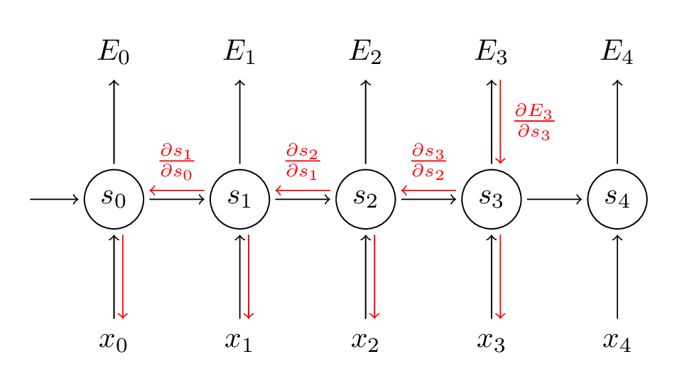
S represets the internal state of the RNN where E is the error/loss and x’s are inputs. Let’s say we are at timestamp 3 and we want to calculate loss how would we go about it.
\[\frac{\partial E_3(w)}{\partial w} = -\frac{\partial log(y_{3c})}{\partial w}\]We know that Yi is dependent on the Si-1 hence by chain rule we can break this down into.
\[\frac{\partial E_3(w)}{\partial w} = -\frac{\partial log(y_{3c})}{\partial S_3} \cdot \frac{\partial S_3}{\partial w}\]Now the first part of the equation is straing forward as eqation of Y3 is present for us with S3 but the second half we have S3 which is depedent on both W ans S 2 which again will be depedent on W. Hence in the equation of S3 S 2 can not be assumed to constant with respect to W.
In such a network total derivate of \(\frac{\partial S_3}{\partial w}\) has two components which is explicite with \(\dagger\) where everthing apart from W is treated as constant and implicite part where we take the derivate with respect to the vaiable which was dependent on W.
\[\frac{\partial S_3}{\partial w} = \frac{\partial^\dagger S_3}{\partial w} + \frac{\partial S_3}{\partial S_2} \cdot \frac{\partial S_2}{\partial w}\]Now we see that we would have to calculated this again for \(\frac{\partial S_2}{\partial w}\) but in practice this is approximated with
\[\frac{\partial S_T}{\partial w} = \sum_{k=1}^{T}\frac{\partial S_T}{\partial S_k} \cdot \frac{\partial ^\dagger S_k}{\partial w}\]Vanishing and Exploding Gradients
If we look at the formula above it has a term \(\frac{\partial S_T}{\partial S_k}\) this is important because as the lenght of the inputs/ouputs increase the we observe a chain of partial derivaties.
\[\frac{\partial S_T}{\partial S_k} = \frac{\partial S_T}{\partial S_{T-1}}\cdot\frac{\partial S_{T-1}}{\partial S_{T-2}}.......\frac{\partial S_{k+1}}{\partial S_{k}}\]For the above equation we have a bound on its value which is \(\prod_{j=k+1}^{T} \gamma.\lambda\) now if \(\gamma.\lambda < 1\) we see vanishing gradients and for when \(\gamma.\lambda>1\) we see exploding gradients. Trucation and gradient clipping are the two brute fore approches to stop such behavior.
This becomes problem because the commbinted effects of the output on longer sequences is lost in case of vanashing gradients. Even though the weights are the same throughout the abilty of RNN’s to produce good results at longer inputs and outputs is hampered.
LSTM
LSMT is a special type of RNN which is designed to avoid the vanishing gradient problem (Note: Both LSTM and RNN can be stacked). The core idea is to intoduce cell state and hidden state indepedent to each other.The only opration that are begin done on the cell state are linear in nature hence the gradient flow does not vanish in exponential nature Proof hence cell state is able to reduce the problem of vanishing gradient. This does not solve the problem of long sequences completely but increase the length at which these networks can work with reasonable accuracy. The digram below helps in understanding the internals of LSTM it has gates which can be summarizes using the follwing keys terms. Forget Gate: The idea is that we want to selectly forget some of the information which is being passed on in the cell state this is done based on the hidden state passed through a linear and a sigmoid which is then multiplied(Hadamat Product) with the cell state. Next we see the Input Gate: which can be seen as Selective Write on the cell state the oprations can seen in the digram. Next come the Output Gate: the ouput gate uses the updated cell state and the hidden state to produce the next hidden state. This same hiddne state can be used as output at time state t or we can apply a linear layer on top of this as well.

Bidirectional LSTM
The idea of Bidirectinal LSTM using only unidirectiona inputs might not be the best things as langugae is not unidirectional in nature. For example This is a ___ which can fly with 12 people. If we just try to fill the blank with the context of left then we would have a lot of options but after the context of right the most relevent word would be a plane. Internally it uses the same lstm units.
